34 混合效应模型

I think that the formula language does allow expressions with ‘/’ to represent nested factors but I can’t check right now as there is a fire in the building where my office is located. I prefer to simply write nested factors as factor1 + factor1:factor2.

— Douglas Bates ¹

library(nlme)         # 线性混合效应模型
library(GLMMadaptive) # 广义线性混合效应模型
library(mgcv)         # 广义线性/可加混合效应模型

library(splines)   # 样条
library(cmdstanr)  # 编译采样
library(ggplot2)   # 作图
library(bayesplot) # 后验分布
library(loo)       # LOO-CV

library(INLA)      # 近似贝叶斯推断

混合效应模型在心理学、生态学、计量经济学和空间统计学等领域应用十分广泛。线性混合效应模型有多个化身，比如生态学里的分层线性模型（Hierarchical linear Model，简称 HLM），心理学的多水平线性模型（Multilevel Linear Model）。模型名称的多样性正说明它应用的广泛性！混合效应模型内容非常多，非常复杂，因此，本章仅对常见的四种类型提供入门级的实战内容。从频率派和贝叶斯派两个角度介绍模型结构及说明、R 代码或 Stan 代码实现及输出结果解释。

除了 R 语言社区提供的开源扩展包，商业的软件有 Mplus 、ASReml 和 SAS 等，而开源的软件 OpenBUGS 、 JAGS 和 Stan 等。混合效应模型的种类非常多，一部分可以在一些流行的 R 包能力范围内解决，其余可以放在更加灵活、扩展性强的框架 Stan 内解决。因此，本章同时介绍 Stan 框架和一些 R 包。

本章用到 4 个数据集，其中 sleepstudy 和 cbpp 均来自 lme4 包 (Bates 等 2015)，分别用于介绍线性混合效应模型和广义线性混合效应模型，Loblolly 来自 datasets 包，用于介绍非线性混合效应模型，最后，朗格拉普岛核辐射数据数据集用于介绍广义可加混合效应模型。

在介绍理论的同时给出 R 语言或 S 语言实现的几本参考书籍。

《Mixed-Effects Models in S and S-PLUS》(Pinheiro 和 Bates 2000)
《Mixed Models: Theory and Applications with R》(Demidenko 2013)
《Linear Mixed-Effects Models Using R: A Step-by-Step Approach》(Gałecki 和 Burzykowski 2013)
《Linear and Generalized Linear Mixed Models and Their Applications》(Jiang 和 Nguyen 2021)

34.1 线性混合效应模型

I think what we are seeking is the marginal variance-covariance matrix of the parameter estimators (marginal with respect to the random effects random variable, B), which would have the form of the inverse of the crossproduct of a \((q+p)\) by \(p\) matrix composed of the vertical concatenation of \(-L^{-1}RZXRX^{-1}\) and \(RX^{-1}\). (Note: You do not want to calculate the first term by inverting \(L\), use solve(L, RZX, system = "L")

[…] don’t even think about using solve(L)

don’t!, don’t!, don’t!

have I made myself clear?

don’t do that (and we all know that someone will do exactly that for a very large \(L\) and then send out messages about “R is SOOOOO SLOOOOW!!!!” :-) )

— Douglas Bates ²

提示

一般的模型结构和假设
一般的模型表达公式
nlme 包的函数 lme()
公式语法和示例模型表示

线性混合效应模型（Linear Mixed Models or Linear Mixed-Effects Models，简称 LME 或 LMM），介绍模型的基础理论，包括一般形式，矩阵表示，参数估计，假设检验，模型诊断，模型评估。参数方法主要是极大似然估计和限制极大似然估计。一般形式如下：

\[ \bm{y} = X\bm{\beta} + Z\bm{u} + \bm{\epsilon} \]

其中，\(\bm{y}\) 是一个向量，代表响应变量，\(X\) 代表固定效应对应的设计矩阵，\(\bm{\beta}\) 是一个参数向量，代表固定效应对应的回归系数，\(Z\) 代表随机效应对应的设计矩阵，\(\bm{u}\) 是一个参数向量，代表随机效应对应的回归系数，\(\bm{\epsilon}\) 表示残差向量。

一般假定随机向量 \(\bm{u}\) 服从多元正态分布，这是无条件分布，随机向量 \(\bm{y}|\bm{u}\) 服从多元正态分布，这是条件分布。

\[ \begin{aligned} \bm{u} &\sim \mathcal{N}(0,\Sigma) \\ \bm{y}|\bm{u} &\sim \mathcal{N}(X\bm{\beta} + Z\bm{u},\sigma^2W) \end{aligned} \]

其中，方差协方差矩阵 \(\Sigma\) 必须是半正定的，\(W\) 是一个对角矩阵。

nlme 和 lme4 等 R 包共用一套表示随机效应的公式语法，如下表所示。

表格 34.1: nlme 包的公式语法
公式	含义
`(1\|group)`	随机组截距
`(x\|group)` = `(1+x\|group)`	变量 x 的随机组斜率和相关截距
`(0+x\|group)` = `(-1+x\|group)`	变量 x 的随机组斜率，无变化的截距
`(1\|group) + (0+x\|group)`	不相关的随机截距，组内随机斜率
`(1\|site/block)` = `(1\|site)+(1\|site:block)`	intercept varying among sites and among blocks within sites (nested random effects)
`site+(1\|site:block)`	fixed effect of sites plus random variation in intercept among blocks within sites
`(x\|site/block)` = `(x\|site)+(x\|site:block)` = `(1 + x\|site)+(1+x\|site:block)`	slope and intercept varying among sites and among blocks within sites
`(x1\|site)+(x2\|block)`	two different effects, varying at different levels
`x*site+(x\|site:block)`	fixed effect variation of slope and intercept varying among sites and random variation of slope and intercept among blocks within sites
`(1\|group1)+(1\|group2)`	intercept varying among crossed random effects (e.g. site, year)

sleepstudy 数据集来自 lme4 包，是一个睡眠研究项目的实验数据。实验对象都是有失眠情况的人，有的人有严重的失眠问题（一天只有 3 个小时的睡眠时间）。进入实验后的前10 天的情况，记录平均反应时间、睡眠不足的天数。

data(sleepstudy, package = "lme4")
str(sleepstudy)

#> 'data.frame':    180 obs. of  3 variables:
#>  $ Reaction: num  250 259 251 321 357 ...
#>  $ Days    : num  0 1 2 3 4 5 6 7 8 9 ...
#>  $ Subject : Factor w/ 18 levels "308","309","310",..: 1 1 1 1 1 1 1 1 1 1 ...

Reaction 表示平均反应时间（毫秒），数值型，Days 表示进入实验后的第几天，数值型，Subject 表示参与实验的个体编号，因子型。

xtabs(~ Days + Subject, data = sleepstudy)

#>     Subject
#> Days 308 309 310 330 331 332 333 334 335 337 349 350 351 352 369 370 371 372
#>    0   1   1   1   1   1   1   1   1   1   1   1   1   1   1   1   1   1   1
#>    1   1   1   1   1   1   1   1   1   1   1   1   1   1   1   1   1   1   1
#>    2   1   1   1   1   1   1   1   1   1   1   1   1   1   1   1   1   1   1
#>    3   1   1   1   1   1   1   1   1   1   1   1   1   1   1   1   1   1   1
#>    4   1   1   1   1   1   1   1   1   1   1   1   1   1   1   1   1   1   1
#>    5   1   1   1   1   1   1   1   1   1   1   1   1   1   1   1   1   1   1
#>    6   1   1   1   1   1   1   1   1   1   1   1   1   1   1   1   1   1   1
#>    7   1   1   1   1   1   1   1   1   1   1   1   1   1   1   1   1   1   1
#>    8   1   1   1   1   1   1   1   1   1   1   1   1   1   1   1   1   1   1
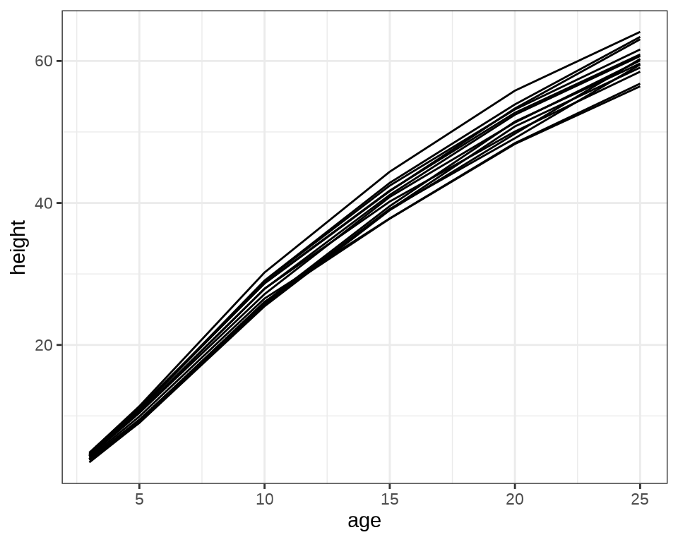
#>    9   1   1   1   1   1   1   1   1   1   1   1   1   1   1   1   1   1   1

每个个体每天产生一条数据，下 @fig-sleepstudy-line 中每条折线代表一个个体。

library(ggplot2)
ggplot(data = sleepstudy, aes(x = Days, y = Reaction, group = Subject)) +
  geom_line() +
  scale_x_continuous(n.breaks = 6) +
  theme_bw() +
  labs(x = "睡眠不足的天数", y = "平均反应时间")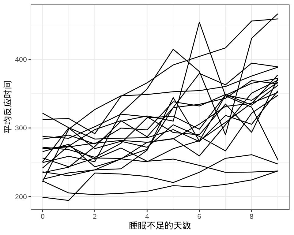

对于连续重复测量的数据（continuous repeated measurement outcomes），也叫纵向数据（longitudinal data），针对不同个体 Subject，相比于上图，下面绘制反应时间 Reaction 随睡眠时间 Days 的变化趋势更合适。图中趋势线是简单线性回归的结果，分面展示不同个体Subject 之间对比。

ggplot(data = sleepstudy, aes(x = Days, y = Reaction)) +
  geom_point() +
  geom_smooth(formula = "y ~ x", method = "lm", se = FALSE) +
  scale_x_continuous(n.breaks = 6) +
  theme_bw() +
  facet_wrap(facets = ~Subject, labeller = "label_both", ncol = 6) +
  labs(x = "睡眠不足的天数", y = "平均反应时间")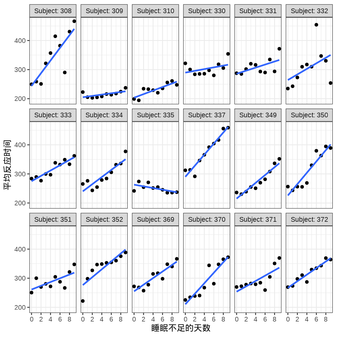

考虑两水平的混合效应模型，其中随机截距 \(\beta_{0j}\) 和随机斜率 \(\beta_{1j}\)，指标 \(j\) 表示分组的编号，也叫变截距和变斜率模型

\[ \begin{aligned} \mathrm{Reaction}_{ij} &= \beta_{0j} + \beta_{1j} \cdot \mathrm{Days}_{ij} + \epsilon_{ij} \\ \beta_{0j} &= \gamma_{00} + U_{0j} \\ \beta_{1j} &= \gamma_{10} + U_{1j} \\ \begin{pmatrix} U_{0j} \\ U_{1j} \end{pmatrix} &\sim \mathcal{N} \begin{bmatrix} \begin{pmatrix} 0 \\ 0 \end{pmatrix} , \begin{pmatrix} \tau^2_{00} & \tau_{01} \\ \tau_{01} & \tau^2_{10} \end{pmatrix} \end{bmatrix} \\ \epsilon_{ij} &\sim \mathcal{N}(0, \sigma^2) \\ i = 0,1,\cdots,9 &\quad j = 308,309,\cdots, 372. \end{aligned} \]

下面用 nlme 包 (Pinheiro 和 Bates 2000) 拟合模型。

library(nlme)
fm1 <- lme(Reaction ~ Days, random = ~ Days | Subject, data = sleepstudy)
summary(fm1)

#> Linear mixed-effects model fit by REML
#>   Data: sleepstudy 
#>        AIC      BIC    logLik
#>   1755.628 1774.719 -871.8141
#> 
#> Random effects:
#>  Formula: ~Days | Subject
#>  Structure: General positive-definite, Log-Cholesky parametrization
#>             StdDev    Corr  
#> (Intercept) 24.740241 (Intr)
#> Days         5.922103 0.066 
#> Residual    25.591843       
#> 
#> Fixed effects:  Reaction ~ Days 
#>                 Value Std.Error  DF  t-value p-value
#> (Intercept) 251.40510  6.824516 161 36.83853       0
#> Days         10.46729  1.545783 161  6.77151       0
#>  Correlation: 
#>      (Intr)
#> Days -0.138
#> 
#> Standardized Within-Group Residuals:
#>         Min          Q1         Med          Q3         Max 
#> -3.95355735 -0.46339976  0.02311783  0.46339621  5.17925089 
#> 
#> Number of Observations: 180
#> Number of Groups: 18

随机效应（Random effects）部分：

# 前 6 个 subject
head(ranef(fm1))

#>     (Intercept)       Days
#> 308    2.258754  9.1989366
#> 309  -40.398490 -8.6197167
#> 310  -38.960098 -5.4489048
#> 330   23.690228 -4.8142826
#> 331   22.259981 -3.0698548
#> 332    9.039458 -0.2721585

固定效应（Fixed effects）部分：

fixef(fm1)

#> (Intercept)        Days 
#>   251.40510    10.46729

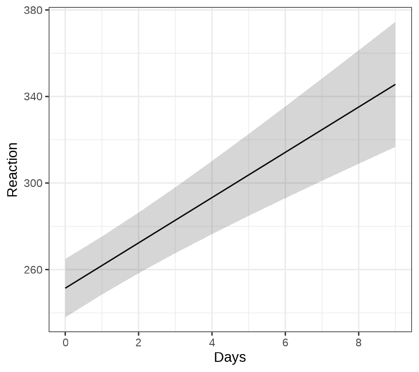
ggeffects 包的函数 ggpredict() 和 ggeffect() 可以用来绘制混合效应模型的边际效应（ Marginal Effects），ggPMX 包可以用来绘制混合效应模型的诊断图。下图 34.3 展示关于变量 Days 的边际效应图。

library(ggeffects)
mydf <- ggpredict(fm1, terms = "Days")
ggplot(mydf, aes(x = x, y = predicted)) +
  geom_line() +
  geom_ribbon(aes(ymin = conf.low, ymax = conf.high), alpha = 0.2) +
  scale_x_continuous(n.breaks = 6) +
  theme_bw() +
  labs(x = "Days", y = "Reaction")

brms

代码

library(brms)
# predictions
fit_sleep2 <- brm(Reaction ~ Days + (Days | Subject), data = sleepstudy)

conds <- make_conditions(fit_sleep2, "Subject")

fit_sleep2 |>
  marginal_effects(
    re_formula = NULL,
    conditions = conds
  ) |>
  plot(points = TRUE, ncol = 6)

34.2 广义线性混合效应模型

当响应变量分布不再是高斯分布，线性混合效应模型就扩展到广义线性混合效应模型。有一些 R 包可以拟合此类模型，MASS 包的函数 glmmPQL() ，lme4 包的函数 glmer() ，GLMMadaptive 包的函数 mixed_model() ，brms 包的函数 brm() 等。

表格 34.2: 响应变量的分布
响应变量分布	MASS	lme4	GLMMadaptive	brms
伯努利分布	支持	支持	支持	支持
二项分布	支持	支持	支持	支持
泊松分布	支持	支持	支持	支持
负二项分布	不支持	支持	支持	支持
伽马分布	支持	支持	支持	支持

函数 glmmPQL() 支持的分布族见函数 glm() 的参数 family ，lme4 包的函数 glmer.nb() 和 GLMMadaptive 包的函数 negative.binomial() 都可用于拟合响应变量服从负二项分布的情况。除了这些常规的分布，GLMMadaptive 和 brms 包还支持许多常见的分布，比如零膨胀的泊松分布、二项分布等，还可以自定义分布。

伯努利分布 family = binomial(link = "logit")
二项分布 family = binomial(link = "logit")
泊松分布 family = poisson(link = "log")
负二项分布 lme4::glmer.nb() 或 GLMMadaptive::negative.binomial()
伽马分布 family = Gamma(link = "inverse")

GLMMadaptive 包 (Rizopoulos 2023) 的主要函数 mixed_model() 是用来拟合广义线性混合效应模型的。下面以牛传染性胸膜肺炎（Contagious bovine pleuropneumonia，简称 CBPP）数据 cbpp 介绍函数 mixed_model() 的用法，该数据集来自 lme4 包。

data(cbpp, package = "lme4")
str(cbpp)

#> 'data.frame':    56 obs. of  4 variables:
#>  $ herd     : Factor w/ 15 levels "1","2","3","4",..: 1 1 1 1 2 2 2 3 3 3 ...
#>  $ incidence: num  2 3 4 0 3 1 1 8 2 0 ...
#>  $ size     : num  14 12 9 5 22 18 21 22 16 16 ...
#>  $ period   : Factor w/ 4 levels "1","2","3","4": 1 2 3 4 1 2 3 1 2 3 ...

herd 牛群编号，period 时间段，incidence 感染的数量，size 牛群大小。疾病在种群内扩散

ggplot(data = cbpp, aes(x = herd, y = period)) +
  geom_tile(aes(fill = incidence / size)) +
  scale_fill_viridis_c(label = scales::percent_format(), 
                       option = "C", name = "") +
  theme_minimal()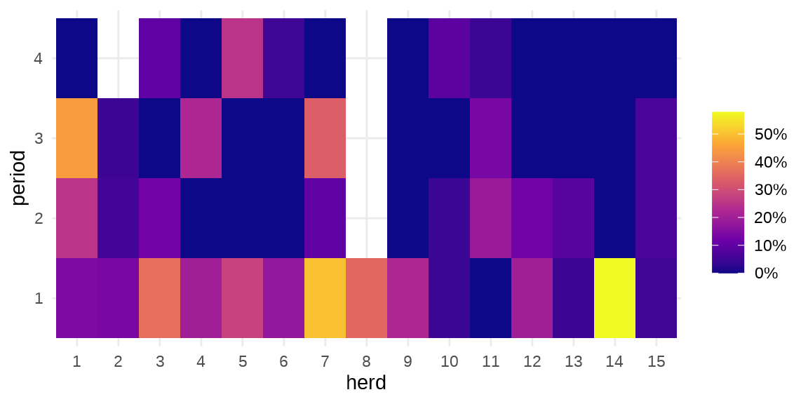

library(GLMMadaptive)
fgm1 <- mixed_model(
  fixed = cbind(incidence, size - incidence) ~ period,
  random = ~ 1 | herd, data = cbpp, family = binomial(link = "logit")
)
summary(fgm1)

#> 
#> Call:
#> mixed_model(fixed = cbind(incidence, size - incidence) ~ period, 
#>     random = ~1 | herd, data = cbpp, family = binomial(link = "logit"))
#> 
#> Data Descriptives:
#> Number of Observations: 56
#> Number of Groups: 15 
#> 
#> Model:
#>  family: binomial
#>  link: logit 
#> 
#> Fit statistics:
#>    log.Lik      AIC     BIC
#>  -91.98337 193.9667 197.507
#> 
#> Random effects covariance matrix:
#>                StdDev
#> (Intercept) 0.6475934
#> 
#> Fixed effects:
#>             Estimate Std.Err z-value    p-value
#> (Intercept)  -1.3995  0.2335 -5.9923    < 1e-04
#> period2      -0.9914  0.3068 -3.2316 0.00123091
#> period3      -1.1278  0.3268 -3.4513 0.00055793
#> period4      -1.5795  0.4276 -3.6937 0.00022101
#> 
#> Integration:
#> method: adaptive Gauss-Hermite quadrature rule
#> quadrature points: 11
#> 
#> Optimization:
#> method: EM
#> converged: TRUE

brms

代码

library(brms)
bgm1 <- brm(
  incidence | trials(size) ~ period + (1 | herd),
  data = cbpp, family = binomial(link = "logit")
)

34.3 非线性混合效应模型

Loblolly 数据集来自 R 内置的 datasets 包

ggplot(data = Loblolly, aes(x = age, y = height, group = Seed)) +
  geom_line() +
  theme_bw()

非线性回归

nfm1 <- nls(height ~ SSasymp(age, Asym, R0, lrc),
           data = Loblolly, subset = Seed == 329)
summary(nfm1)

#> 
#> Formula: height ~ SSasymp(age, Asym, R0, lrc)
#> 
#> Parameters:
#>      Estimate Std. Error t value Pr(>|t|)    
#> Asym  94.1282     8.4030  11.202 0.001525 ** 
#> R0    -8.2508     1.2261  -6.729 0.006700 ** 
#> lrc   -3.2176     0.1386 -23.218 0.000175 ***
#> ---
#> Signif. codes:  0 '***' 0.001 '**' 0.01 '*' 0.05 '.' 0.1 ' ' 1
#> 
#> Residual standard error: 0.7493 on 3 degrees of freedom
#> 
#> Number of iterations to convergence: 0 
#> Achieved convergence tolerance: 4.148e-07

非线性函数 SSasymp() 的内容如下

\[ \mathrm{Asym}+(\mathrm{R0}-\mathrm{Asym})\times\exp\big(-\exp(\mathrm{lrc})\times\mathrm{input}\big) \]

其中，\(\mathrm{Asym}\) 、\(\mathrm{R0}\) 、\(\mathrm{lrc}\) 是参数，\(\mathrm{input}\) 是输入值。

示例来自 nlme 包的函数 nlme() 帮助文档

nfm2 <- nlme(height ~ SSasymp(age, Asym, R0, lrc),
  data = Loblolly,
  fixed = Asym + R0 + lrc ~ 1,
  random = Asym ~ 1,
  start = c(Asym = 103, R0 = -8.5, lrc = -3.3)
)
summary(nfm2)

#> Nonlinear mixed-effects model fit by maximum likelihood
#>   Model: height ~ SSasymp(age, Asym, R0, lrc) 
#>   Data: Loblolly 
#>        AIC      BIC    logLik
#>   239.4856 251.6397 -114.7428
#> 
#> Random effects:
#>  Formula: Asym ~ 1 | Seed
#>             Asym  Residual
#> StdDev: 3.650642 0.7188625
#> 
#> Fixed effects:  Asym + R0 + lrc ~ 1 
#>          Value Std.Error DF   t-value p-value
#> Asym 101.44960 2.4616951 68  41.21128       0
#> R0    -8.62733 0.3179505 68 -27.13420       0
#> lrc   -3.23375 0.0342702 68 -94.36052       0
#>  Correlation: 
#>     Asym   R0    
#> R0   0.704       
#> lrc -0.908 -0.827
#> 
#> Standardized Within-Group Residuals:
#>         Min          Q1         Med          Q3         Max 
#> -2.23601930 -0.62380854  0.05917466  0.65727206  1.95794425 
#> 
#> Number of Observations: 84
#> Number of Groups: 14

# 更新模型的随机效应部分
nfm3 <- update(nfm2, random = pdDiag(Asym + lrc ~ 1))
summary(nfm3)

#> Nonlinear mixed-effects model fit by maximum likelihood
#>   Model: height ~ SSasymp(age, Asym, R0, lrc) 
#>   Data: Loblolly 
#>        AIC      BIC    logLik
#>   238.9662 253.5511 -113.4831
#> 
#> Random effects:
#>  Formula: list(Asym ~ 1, lrc ~ 1)
#>  Level: Seed
#>  Structure: Diagonal
#>             Asym        lrc  Residual
#> StdDev: 2.806185 0.03449969 0.6920003
#> 
#> Fixed effects:  Asym + R0 + lrc ~ 1 
#>          Value Std.Error DF   t-value p-value
#> Asym 101.85205 2.3239828 68  43.82651       0
#> R0    -8.59039 0.3058441 68 -28.08747       0
#> lrc   -3.24011 0.0345017 68 -93.91167       0
#>  Correlation: 
#>     Asym   R0    
#> R0   0.727       
#> lrc -0.902 -0.796
#> 
#> Standardized Within-Group Residuals:
#>         Min          Q1         Med          Q3         Max 
#> -2.06072906 -0.69785679  0.08721706  0.73687722  1.79015782 
#> 
#> Number of Observations: 84
#> Number of Groups: 14

brms

代码

library(brms)
lob_prior <- c(
  set_prior("normal(101, 0.1)", nlpar = "Asym", lb = 100, ub = 102),
  set_prior("normal(-8, 1)", nlpar = "R0", lb = -10),
  set_prior("normal(-3, 3)", nlpar = "lrc", lb = -9),
  set_prior("normal(3, 0.2)", class = "sigma")
)

lob_formula <- bf(
  height ~ Asym + (R0 - Asym) * exp( - exp(lrc) * age),
  # Nonlinear variables
  # Fixed effects: Asym R0 lrc
  R0 + lrc ~ 1,
  # Nonlinear variables
  # Random effects: Seed
  Asym ~ 1 + (1 | Seed),
  # Nonlinear fit
  nl = TRUE
)

lob_bayes_fit <- brm(
  lob_formula, family = gaussian(), data = Loblolly, prior = lob_prior
)

34.4 广义可加混合效应模型

从线性到可加，意味着从线性到非线性，可加模型容纳非线性的成分，比如高斯过程、样条。

34.4.1 mgcv

本节复用章节 27 朗格拉普岛核污染数据，相关背景不再赘述，下面首先加载数据到 R 环境。

# 加载数据
rongelap <- readRDS(file = "data/rongelap.rds")
rongelap_coastline <- readRDS(file = "data/rongelap_coastline.rds")

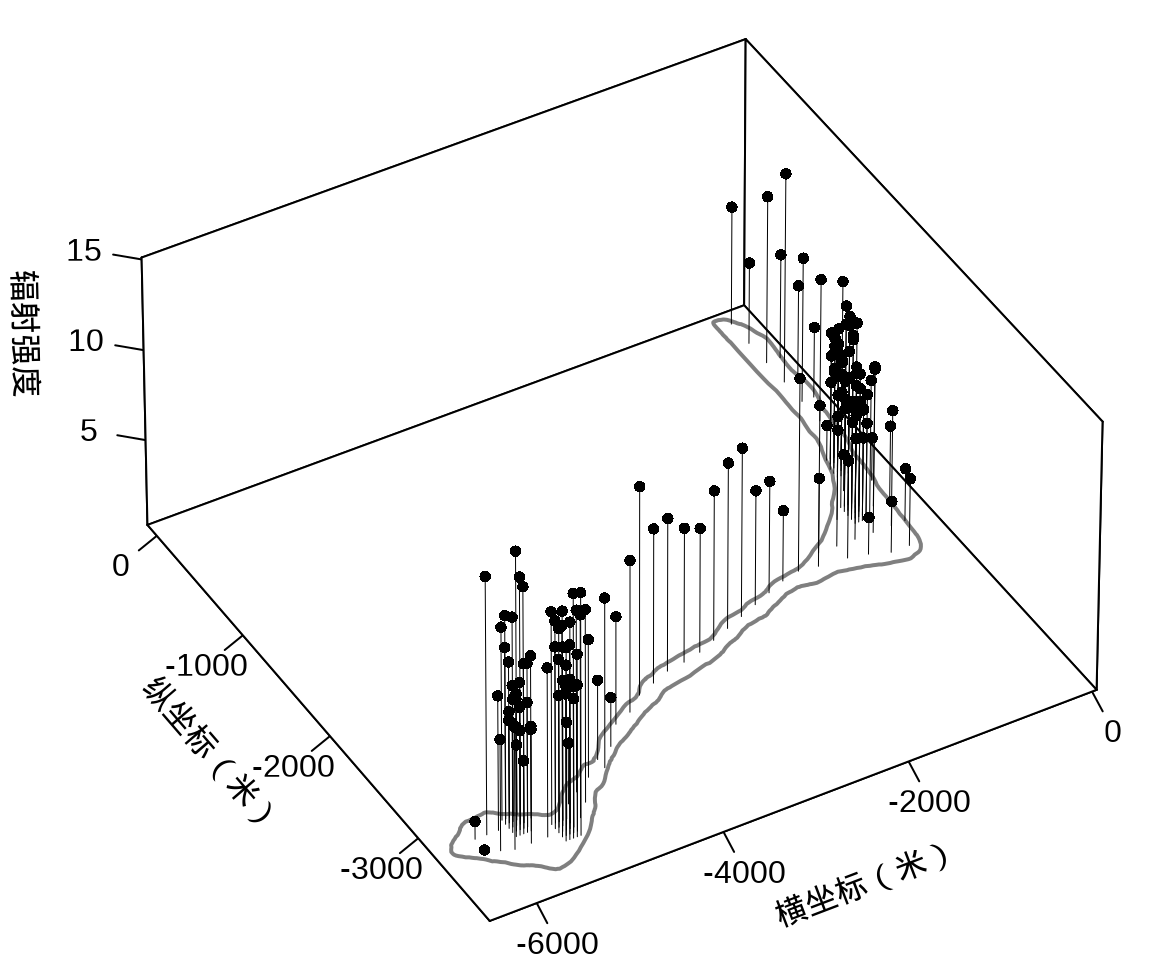
接着，将岛上各采样点的辐射强度展示出来，算是简单回顾一下数据概况。

代码

library(plot3D)
with(rongelap, {
  opar <- par(mar = c(.1, 2.5, .1, .1), no.readonly = TRUE)
  rongelap_coastline$cZ <- 0
  scatter3D(
    x = cX, y = cY, z = counts / time, 
    xlim = c(-6500, 50), ylim = c(-3800, 110),
    xlab = "\n横坐标（米）", ylab = "\n纵坐标（米）",
    zlab = "\n辐射强度", lwd = 0.5, cex = 0.8,
    pch = 16, type = "h", ticktype = "detailed",
    phi = 40, theta = -30, r = 50, d = 1,
    expand = 0.5, box = TRUE, bty = "b",
    colkey = F, col = "black",
    panel.first = function(trans) {
      XY <- trans3D(
        x = rongelap_coastline$cX,
        y = rongelap_coastline$cY,
        z = rongelap_coastline$cZ,
        pmat = trans
      )
      lines(XY, col = "gray50", lwd = 2)
    }
  )
  rongelap_coastline$cZ <- NULL
  on.exit(par(opar), add = TRUE)
})

在这里，从广义可加混合效应模型的角度来对核污染数据建模，空间效应仍然是用高斯过程来表示，响应变量服从带漂移项的泊松分布。采用 mgcv 包 (Wood 2004) 的函数 gam() 拟合模型，其中，含 49 个参数的样条近似高斯过程，高斯过程的核函数为默认的梅隆型。更多详情见 mgcv 包的函数 s() 帮助文档参数的说明，默认值是梅隆型相关函数及默认的范围参数，作者自己定义了一套符号约定。

library(nlme)
library(mgcv)
fit_rongelap_gam <- gam(
  counts ~ s(cX, cY, bs = "gp", k = 50), offset = log(time), 
  data = rongelap, family = poisson(link = "log")
)
# 模型输出
summary(fit_rongelap_gam)

#> 
#> Family: poisson 
#> Link function: log 
#> 
#> Formula:
#> counts ~ s(cX, cY, bs = "gp", k = 50)
#> 
#> Parametric coefficients:
#>             Estimate Std. Error z value Pr(>|z|)    
#> (Intercept) 1.976815   0.001642    1204   <2e-16 ***
#> ---
#> Signif. codes:  0 '***' 0.001 '**' 0.01 '*' 0.05 '.' 0.1 ' ' 1
#> 
#> Approximate significance of smooth terms:
#>            edf Ref.df Chi.sq p-value    
#> s(cX,cY) 48.98     49  34030  <2e-16 ***
#> ---
#> Signif. codes:  0 '***' 0.001 '**' 0.01 '*' 0.05 '.' 0.1 ' ' 1
#> 
#> R-sq.(adj) =  0.876   Deviance explained = 60.7%
#> UBRE = 153.78  Scale est. = 1         n = 157

# 随机效应
gam.vcomp(fit_rongelap_gam)

#> s(cX,cY) 
#> 2543.376

值得一提的是核函数的类型和默认参数的选择，参数 m 接受一个向量， m[1] 取值为 1 至 5，分别代表球型 spherical, 幂指数 power exponential 和梅隆型 Matern with \(\kappa\) = 1.5, 2.5 or 3.5 等 5 种相关/核函数。

# 球型相关函数及范围参数为 0.5
fit_rongelap_gam <- gam(
  counts ~ s(cX, cY, bs = "gp", k = 50, m = c(1, .5)),
  offset = log(time), data = rongelap, family = poisson(link = "log")
)

接下来，基于岛屿的海岸线数据划分出网格，将格点作为新的预测位置。

library(sf)

#> Linking to GEOS 3.11.1, GDAL 3.6.4, PROJ 9.1.1; sf_use_s2() is TRUE

library(abind)
library(stars)
# 类型转化
rongelap_sf <- st_as_sf(rongelap, coords = c("cX", "cY"), dim = "XY")
rongelap_coastline_sf <- st_as_sf(rongelap_coastline, coords = c("cX", "cY"), dim = "XY")
rongelap_coastline_sfp <- st_cast(st_combine(st_geometry(rongelap_coastline_sf)), "POLYGON")
# 添加缓冲区
rongelap_coastline_buffer <- st_buffer(rongelap_coastline_sfp, dist = 50)
# 构造带边界约束的网格
rongelap_coastline_grid <- st_make_grid(rongelap_coastline_buffer, n = c(150, 75))
# 将 sfc 类型转化为 sf 类型
rongelap_coastline_grid <- st_as_sf(rongelap_coastline_grid)
rongelap_coastline_buffer <- st_as_sf(rongelap_coastline_buffer)
rongelap_grid <- rongelap_coastline_grid[rongelap_coastline_buffer, op = st_intersects]
# 计算网格中心点坐标
rongelap_grid_centroid <- st_centroid(rongelap_grid)
# 共计 1612 个预测点
rongelap_grid_df <- as.data.frame(st_coordinates(rongelap_grid_centroid))
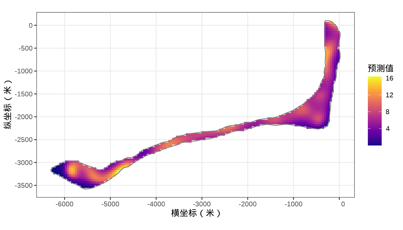
colnames(rongelap_grid_df) <- c("cX", "cY")

模型对象 fit_rongelap_gam 在新的格点上预测核辐射强度，接着整理预测结果数据。

# 预测
rongelap_grid_df$ypred <- as.vector(predict(fit_rongelap_gam, newdata = rongelap_grid_df, type = "response")) 
# 整理预测数据
rongelap_grid_sf <- st_as_sf(rongelap_grid_df, coords = c("cX", "cY"), dim = "XY")
rongelap_grid_stars <- st_rasterize(rongelap_grid_sf, nx = 150, ny = 75)
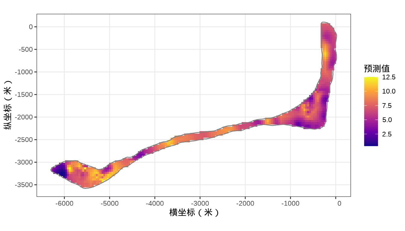
rongelap_stars <- st_crop(x = rongelap_grid_stars, y = rongelap_coastline_sfp)

最后，将岛上各个格点的核辐射强度绘制出来，给出全岛核辐射强度的空间分布。

代码

library(ggplot2)
ggplot() +
  geom_stars(data = rongelap_stars, aes(fill = ypred), na.action = na.omit) +
  geom_sf(data = rongelap_coastline_sfp, fill = NA, color = "gray50", linewidth = 0.5) +
  scale_fill_viridis_c(option = "C") +
  theme_bw() +
  labs(x = "横坐标（米）", y = "纵坐标（米）", fill = "预测值")

brms

代码

library(brms)
# 预计运行 1 个小时以上
rongelap_brm <- brm(counts ~ gp(cX, cY) + offset(log(time)),
  data = rongelap, family = poisson(link = "log")
)
# 50 个基函数 computing approximate GPs.
rongelap_brm <- brm(
  counts ~ gp(cX, cY, c = 5/4, k = 50) + offset(log(time)),
  data = rongelap, family = poisson(link = "log")
)

34.4.2 INLA

mgcv 包的函数 ginla() 实现简化版的 Integrated Nested Laplace Approximation, INLA (Rue, Martino, 和 Chopin 2009)。

rongelap_gam <- gam(
  counts ~ s(cX, cY, bs = "gp", k = 50), offset = log(time), 
  data = rongelap, family = poisson(link = "log"), fit = FALSE
)
# 简化版 INLA
fit_rongelap_ginla <- ginla(G = rongelap_gam)
str(fit_rongelap_ginla)

#> List of 2
#>  $ density: num [1:50, 1:100] 2.49e-01 9.03e-06 3.51e-06 1.97e-06 1.17e-06 ...
#>  $ beta   : num [1:50, 1:100] 1.97 -676.61 -572.67 4720.77 240.12 ...

其中， \(k = 50\) 表示 49 个样条参数，每个参数的分布对应有 100 个采样点，另外，截距项的边际后验概率密度分布如下：

plot(
  fit_rongelap_ginla$beta[1, ], fit_rongelap_ginla$density[1, ],
  type = "l", xlab = "截距项", ylab = "概率密度"
)

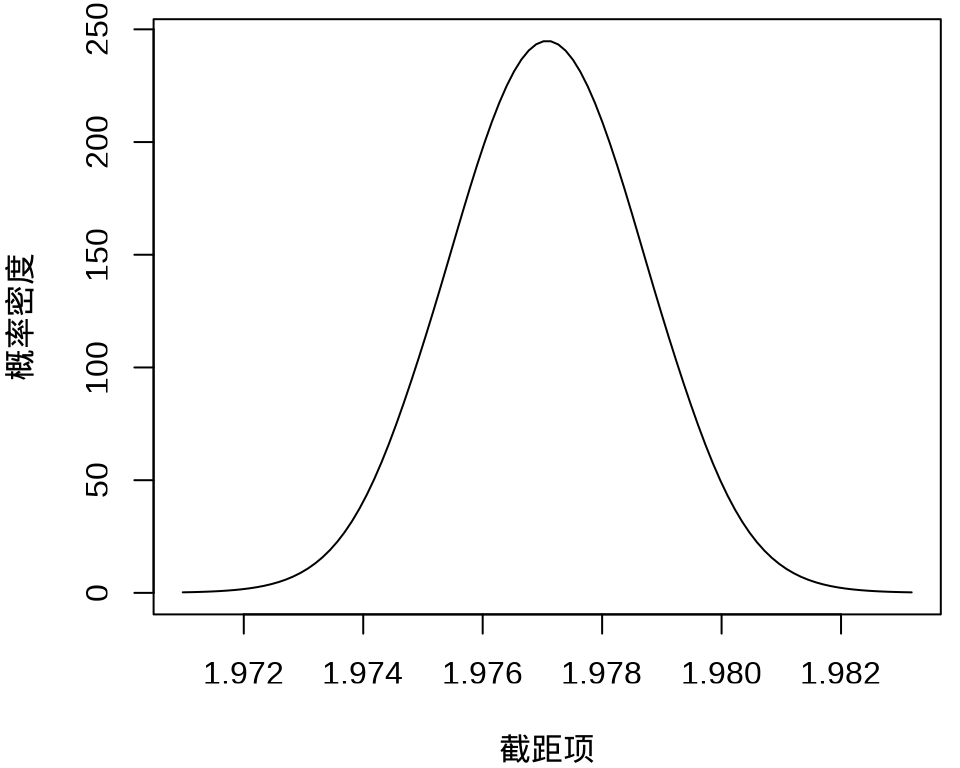
不难看出，截距项在 1.976 至 1.978 之间，50个参数的最大后验估计分别如下：

idx <- apply(fit_rongelap_ginla$density, 1, function(x) x == max(x))
fit_rongelap_ginla$beta[t(idx)]

#>  [1]  1.977019e+00 -5.124099e+02  5.461183e+03  1.515296e+03 -2.822166e+03
#>  [6] -1.598371e+04 -6.417855e+03  1.938122e+02 -4.270878e+03  3.769951e+03
#> [11] -1.002035e+04  1.914717e+03 -9.721572e+03 -3.794461e+04 -1.401549e+04
#> [16] -5.376582e+04 -1.585899e+04 -2.338235e+04  6.239053e+04 -3.574501e+02
#> [21] -4.587927e+04  1.723604e+04 -4.514781e+03  9.184026e-02  3.496526e-01
#> [26] -1.477406e+02  4.585057e+03  9.153647e+03  1.929387e+04 -1.116512e+04
#> [31] -1.166149e+04  8.079451e+02  3.627369e+03 -9.835680e+03  1.357777e+04
#> [36]  1.487742e+04  3.880562e+04 -1.708858e+03  2.775844e+04  2.527415e+04
#> [41] -3.932957e+04  3.548123e+04 -1.116341e+04  1.630910e+04 -9.789381e+02
#> [46] -2.011250e+04  2.699657e+04 -4.744393e+04  2.753347e+04  2.834356e+04

接下来，介绍完整版的近似贝叶斯推断方法 INLA — 集成嵌套拉普拉斯近似 (Integrated Nested Laplace Approximations，简称 INLA) (Rue, Martino, 和 Chopin 2009)。根据研究区域的边界构造非凸的内外边界，处理边界效应。

library(INLA)
library(splancs)
# 构造非凸的边界
boundary <- list(
  inla.nonconvex.hull(
    points = as.matrix(rongelap_coastline[,c("cX", "cY")]), 
    convex = 100, concave = 150, resolution = 100),
  inla.nonconvex.hull(
    points = as.matrix(rongelap_coastline[,c("cX", "cY")]), 
    convex = 200, concave = 200, resolution = 200)
)

根据研究区域的情况构造网格，边界内部三角网格最大边长为 300，边界外部最大边长为 600，边界外凸出距离为 100 米。

# 构造非凸的网格
mesh <- inla.mesh.2d(
  loc = as.matrix(rongelap[, c("cX", "cY")]), offset = 100,
  max.edge = c(300, 600), boundary = boundary
)

构建 SPDE，指定自协方差函数为指数型，则 \(\nu = 1/2\) ，因是二维平面，则 \(d = 2\) ，根据 \(\alpha = \nu + d/2\) ，从而 alpha = 3/2 。

spde <- inla.spde2.matern(mesh = mesh, alpha = 3/2, constr = TRUE)

生成 SPDE 模型的指标集，也是随机效应部分。

indexs <- inla.spde.make.index(name = "s", n.spde = spde$n.spde)
lengths(indexs)

#>       s s.group  s.repl 
#>     691     691     691

投影矩阵，三角网格和采样点坐标之间的投影。观测数据 rongelap 和未采样待预测的位置数据 rongelap_grid_df

# 观测位置投影到三角网格上
A <- inla.spde.make.A(mesh = mesh, loc = as.matrix(rongelap[, c("cX", "cY")]) )
# 预测位置投影到三角网格上
coop <- as.matrix(rongelap_grid_df[, c("cX", "cY")])
Ap <- inla.spde.make.A(mesh = mesh, loc = coop)
# 1612 个预测位置
dim(Ap)

#> [1] 1612  691

准备观测数据和预测位置，构造一个 INLA 可以使用的数据栈 Data Stack。

# 在采样点的位置上估计 estimation stk.e
stk.e <- inla.stack(
  tag = "est",
  data = list(y = rongelap$counts, E = rongelap$time),
  A = list(rep(1, 157), A),
  effects = list(data.frame(b0 = 1), s = indexs)
)

# 在新生成的位置上预测 prediction stk.p
stk.p <- inla.stack(
  tag = "pred",
  data = list(y = NA, E = NA),
  A = list(rep(1, 1612), Ap),
  effects = list(data.frame(b0 = 1), s = indexs)
)

# 合并数据 stk.full has stk.e and stk.p
stk.full <- inla.stack(stk.e, stk.p)

指定响应变量与漂移项、联系函数、模型公式。

# 模型拟合
res <- inla(formula = y ~ 0 + b0 + f(s, model = spde),
  data = inla.stack.data(stk.full),
  E = E, # E 已知漂移项
  control.family = list(link = "log"),
  control.predictor = list(
    compute = TRUE, 
    link = 1, # 与 control.family 联系函数相同
    A = inla.stack.A(stk.full)
  ),
  control.compute = list(
    cpo = TRUE, 
    waic = TRUE, # WAIC 统计量 通用信息准则
    dic = TRUE   # DIC 统计量 偏差信息准则
  ),
  family = "poisson"
)
# 模型输出
summary(res)

#> 
#> Call:
#>    c("inla.core(formula = formula, family = family, contrasts = contrasts, 
#>    ", " data = data, quantiles = quantiles, E = E, offset = offset, ", " 
#>    scale = scale, weights = weights, Ntrials = Ntrials, strata = strata, 
#>    ", " lp.scale = lp.scale, link.covariates = link.covariates, verbose = 
#>    verbose, ", " lincomb = lincomb, selection = selection, control.compute 
#>    = control.compute, ", " control.predictor = control.predictor, 
#>    control.family = control.family, ", " control.inla = control.inla, 
#>    control.fixed = control.fixed, ", " control.mode = control.mode, 
#>    control.expert = control.expert, ", " control.hazard = control.hazard, 
#>    control.lincomb = control.lincomb, ", " control.update = 
#>    control.update, control.lp.scale = control.lp.scale, ", " 
#>    control.pardiso = control.pardiso, only.hyperparam = only.hyperparam, 
#>    ", " inla.call = inla.call, inla.arg = inla.arg, num.threads = 
#>    num.threads, ", " keep = keep, working.directory = working.directory, 
#>    silent = silent, ", " inla.mode = inla.mode, safe = FALSE, debug = 
#>    debug, .parent.frame = .parent.frame)" ) 
#> Time used:
#>     Pre = 1.21, Running = 2.39, Post = 0.0993, Total = 3.7 
#> Fixed effects:
#>     mean    sd 0.025quant 0.5quant 0.975quant  mode kld
#> b0 1.828 0.061      1.706    1.828      1.948 1.828   0
#> 
#> Random effects:
#>   Name     Model
#>     s SPDE2 model
#> 
#> Model hyperparameters:
#>               mean    sd 0.025quant 0.5quant 0.975quant  mode
#> Theta1 for s  2.00 0.063       1.88     2.00       2.12  2.00
#> Theta2 for s -4.85 0.130      -5.11    -4.85      -4.59 -4.85
#> 
#> Deviance Information Criterion (DIC) ...............: 1834.56
#> Deviance Information Criterion (DIC, saturated) ....: 314.90
#> Effective number of parameters .....................: 156.46
#> 
#> Watanabe-Akaike information criterion (WAIC) ...: 1789.31
#> Effective number of parameters .................: 80.06
#> 
#> Marginal log-Likelihood:  -1331.95 
#> CPO, PIT is computed 
#> Posterior summaries for the linear predictor and the fitted values are computed
#> (Posterior marginals needs also 'control.compute=list(return.marginals.predictor=TRUE)')

kld 表示 Kullback-Leibler divergence (KLD) 它的值描述标准高斯分布与 Simplified Laplace Approximation 之间的差别，值越小越表示拉普拉斯的近似效果好。
DIC 和 WAIC 指标都是评估模型预测表现的。另外，还有两个量计算出来了，但是没有显示，分别是 CPO 和 PIT 。CPO 表示 Conditional Predictive Ordinate (CPO)，PIT 表示 Probability Integral Transforms (PIT) 。

固定效应（截距）和超参数部分

# 截距
res$summary.fixed

#>        mean         sd 0.025quant 0.5quant 0.975quant     mode          kld
#> b0 1.828057 0.06149189   1.706415 1.828314   1.948234 1.828309 1.782794e-08

# 超参数
res$summary.hyperpar

#>                   mean         sd 0.025quant  0.5quant 0.975quant      mode
#> Theta1 for s  2.000465 0.06252205   1.876613  2.000728   2.122784  2.001823
#> Theta2 for s -4.851576 0.12998437  -5.106817 -4.851802  -4.595021 -4.852739

提取预测数据，并整理数据。

# 预测值对应的指标集合
index <- inla.stack.index(stk.full, tag = "pred")$data
# 提取预测结果，后验均值
# pred_mean <- res$summary.fitted.values[index, "mean"]
# 95% 预测下限
# pred_ll <- res$summary.fitted.values[index, "0.025quant"]
# 95% 预测上限
# pred_ul <- res$summary.fitted.values[index, "0.975quant"]
# 整理数据
rongelap_grid_df$ypred <- res$summary.fitted.values[index, "mean"]
# 预测值数据
rongelap_grid_sf <- st_as_sf(rongelap_grid_df, coords = c("cX", "cY"), dim = "XY")
rongelap_grid_stars <- st_rasterize(rongelap_grid_sf, nx = 150, ny = 75)
rongelap_stars <- st_crop(x = rongelap_grid_stars, y = rongelap_coastline_sfp)

最后，类似之前 mgcv 建模的最后一步，将 INLA 的预测结果绘制出来。

ggplot() +
  geom_stars(data = rongelap_stars, aes(fill = ypred), na.action = na.omit) +
  geom_sf(data = rongelap_coastline_sfp, fill = NA, color = "gray50", linewidth = 0.5) +
  scale_fill_viridis_c(option = "C") +
  theme_bw() +
  labs(x = "横坐标（米）", y = "纵坐标（米）", fill = "预测值")

34.5 总结

本章介绍函数 MASS::glmmPQL()、 nlme::lme()、lme4::lmer() 和 brms::brm() 的用法，以及它们求解线性混合效应模型的区别和联系。在贝叶斯估计方法中，brms 包和 INLA 包都支持非常丰富的模型种类，前者是贝叶斯精确推断，后者是贝叶斯近似推断，brms 基于概率编程语言 Stan 框架打包了许多模型的 Stan 实现，INLA 基于求解随机偏微分方程的有限元方法和拉普拉斯近似技巧，将各类常见统计模型统一起来，计算速度快，计算结果准确。

函数 nlme::lme() 极大似然估计和限制极大似然估计
函数 MASS::glmmPQL() 惩罚拟似然估计，MASS 是依赖 nlme 包， nlme 不支持模型中添加漂移项，所以函数 glmmPQL() 也不支持添加漂移项。
函数 lme4::lmer() 拉普拉斯近似。关于随机效应的高维积分
函数 brms::brm() 汉密尔顿蒙特卡罗抽样。HMC 方法结合自适应步长的采样器 NUTS 来抽样。
函数 INLA::inla() 集成嵌套拉普拉斯近似。

表格 34.3: 混合效应模型及相关 R 包拟合函数
模型	nlme	MASS	lme4	GLMMadaptive	brms
线性混合效应模型	`lme()`	`glmmPQL()`	`lmer()`	不支持	`brm()`
广义线性混合效应模型	不支持	`glmmPQL()`	`glmer()`	`mixed_model()`	`brm()`
非线性混合效应模型	`nlme()`	不支持	`nlmer()`	不支持	`brm()`

通过对频率派和贝叶斯派方法的比较，发现一些有意思的结果。与 Stan 不同，INLA 包做近似贝叶斯推断，计算效率很高。

INLA 软件能处理上千个高斯随机效应，但最多只能处理 15 个超参数，因为 INLA 使用 CCD 处理超参数。如果使用 MCMC 处理超参数，就有可能处理更多的超参数，Daniel Simpson 等把 Laplace approximation 带入 Stan，这样就可以处理上千个超参数。更多理论内容见 2009 年 INLA 诞生的论文和《Advanced Spatial Modeling with Stochastic Partial Differential Equations Using R and INLA》中第一章的估计方法 CCD。

34.6 习题

基于奥克兰火山地形数据集 volcano ，随机拆分成训练数据和测试数据，训练数据可以看作采样点的观测数据，建立高斯过程回归模型，比较测试数据与未采样的位置上的预测数据，在计算速度、准确度、易用性等方面总结 Stan 和 INLA 的特点。

基于 PlantGrowth 数据集，比较将 group 变量视为随机变量与随机效应的异同？

fit_lm <- lm(weight ~ group, data = PlantGrowth)
summary(fit_lm)
fit_lme <- nlme::lme(weight ~ 1, random = ~ 1 | group, data = PlantGrowth)
summary(fit_lme)
fit_lme4 <- lme4::lmer(weight ~ 1 + (1 | group), data = PlantGrowth)
summary(fit_lme4)

从频率派和贝叶斯派角度分别比较多个 R 包对线性混合效应模型的拟合效果。提示：函数 MASS::glmmPQL() 、函数 lme4::lmer()，以及函数 blme::blmer() 和 brms::brm() 。

代码

# 加载数据集
data(sleepstudy, package = "lme4")
fit_lmm_mass <- MASS::glmmPQL(Reaction ~ Days,
  random = ~ Days | Subject, verbose = FALSE,
  data = sleepstudy, family = gaussian
)
summary(fit_lmm_mass)
coef(summary(fit_lmm_mass))

fit_lmm_lme4 <- lme4::lmer(Reaction ~ Days + (Days | Subject), data = sleepstudy)
summary(fit_lmm_lme4)
coef(summary(fit_lmm_lme4))

fit_lmm_blme <- blme::blmer(
  Reaction ~ Days + (Days | Subject), data = sleepstudy,
  control = lme4::lmerControl(check.conv.grad = "ignore"),
  cov.prior = gamma)
summary(fit_lmm_blme)
coef(summary(fit_lmm_blme))

fit_lmm_brms <- brms::brm(Reaction ~ Days + (Days | Subject),
  data = sleepstudy, refresh = 0
)
summary(fit_lmm_brms)

从频率派和贝叶斯派角度分别比较多个 R 包对广义线性混合效应模型的拟合效果。提示：函数 MASS::glmmPQL() 、函数 lme4::glmer() 和函数 glmmTMB::glmmTMB()，以及函数 blme::bglmer() 和函数 brms::brm() 。

代码

# 加载数据集
data(cbpp, package = "lme4")

fit_glmm_mass <- MASS::glmmPQL(
  cbind(incidence, size - incidence) ~ period ,
  random = ~ 1 | herd, verbose = FALSE,
  data = cbpp, family = binomial("logit")
)
summary(fit_glmm_mass)
coef(summary(fit_glmm_mass))

fit_glmm_lme4 <- lme4::glmer(
  cbind(incidence, size - incidence) ~ period + (1 | herd),
  family = binomial("logit"), data = cbpp
)
summary(fit_glmm_lme4)

fit_glmm_glmmtmb <- glmmTMB::glmmTMB(
  cbind(incidence, size - incidence) ~ period + (1 | herd),
  data = cbpp, family = binomial, REML = TRUE
) # REML 估计
summary(fit_glmm_glmmtmb)

fit_glmm_blme <- blme::bglmer(
  cbind(incidence, size - incidence) ~ period + (1 | herd),
  family = binomial("logit"), data = cbpp
)
summary(fit_glmm_blme)

fit_glmm_brms <- brms::brm(
  incidence | trials(size) ~ period + (1 | herd),
  family = binomial("logit"), data = cbpp
)
summary(fit_glmm_brms)

或使用 mgcv 包，可以得到近似的结果。随机效应部分可以看作可加的惩罚项

library(mgcv)
fgm3 <- gam(
  cbind(incidence, size - incidence) ~ period + s(herd, bs = "re"),
  data = cbpp, family = binomial(link = "logit"), method = "REML"
)
summary(fgm3)

#> 
#> Family: binomial 
#> Link function: logit 
#> 
#> Formula:
#> cbind(incidence, size - incidence) ~ period + s(herd, bs = "re")
#> 
#> Parametric coefficients:
#>             Estimate Std. Error z value Pr(>|z|)    
#> (Intercept)  -1.3670     0.2358  -5.799 6.69e-09 ***
#> period2      -0.9693     0.3040  -3.189 0.001428 ** 
#> period3      -1.1045     0.3241  -3.407 0.000656 ***
#> period4      -1.5519     0.4251  -3.651 0.000261 ***
#> ---
#> Signif. codes:  0 '***' 0.001 '**' 0.01 '*' 0.05 '.' 0.1 ' ' 1
#> 
#> Approximate significance of smooth terms:
#>          edf Ref.df Chi.sq  p-value    
#> s(herd) 9.66     14  32.03 3.21e-05 ***
#> ---
#> Signif. codes:  0 '***' 0.001 '**' 0.01 '*' 0.05 '.' 0.1 ' ' 1
#> 
#> R-sq.(adj) =  0.515   Deviance explained =   53%
#> -REML = 93.199  Scale est. = 1         n = 56

下面给出随机效应的标准差的估计及其上下限，和前面 GLMMadaptive 包和 lme4 包给出的结果也是接近的。

gam.vcomp(fgm3)

#> 
#> Standard deviations and 0.95 confidence intervals:
#> 
#>           std.dev     lower    upper
#> s(herd) 0.6818673 0.3953145 1.176135
#> 
#> Rank: 1/1

从广义线性混合效应模型生成模拟数据，用至少 6 个不同的 R 包估计模型参数，比较和归纳不同估计方法和实现算法的效果。举例：带漂移项的泊松型广义线性混合效应模型。\(y_{ij}\) 表示响应变量，\(\bm{u}\) 表示随机效应，\(o_{ij}\) 表示漂移项。

\[ \begin{aligned} y_{ij}|\bm{u} &\sim \mathrm{Poisson}(o_{ij}\lambda_{ij}) \\ \log(\lambda_{ij}) &= \beta_{ij}x_{ij} + u_{j} \\ u_j &\sim \mathcal{N}(0, \sigma^2) \\ i = 1,2,\ldots, n &\quad j = 1,2,\ldots,q \end{aligned} \]

代码

set.seed(2023)
Ngroups <- 25
NperGroup <- 100
# 样本量
N <- Ngroups * NperGroup
# 截距和两个协变量的系数
beta <- c(0.5, 0.3, 0.2)
# 两个协变量
X <- MASS::mvrnorm(N, mu = rep(0, 2), Sigma = matrix(c(1, 0.8, 0.8, 1), 2))
# 漂移项
o <- rep(c(2, 4), each = N / 2)
# 分 25 个组 每个组 100 个观察值
g <- factor(rep(1:Ngroups, each = NperGroup))
u <- rnorm(Ngroups, sd = .5) # 随机效应的标准差 0.5
# 泊松分布的期望
lambda <- o * exp(cbind(1, X) %*% beta + u[g])
# 响应变量的值
y <- rpois(N, lambda = lambda)
# 模拟的数据集
sim_data <- data.frame(y, X, o, g)
colnames(sim_data) <- c("y", "x1", "x2", "o", "g")

# 模型拟合
library(lme4)
fit_sim_poisson_glmer <- glmer(y ~ x1 + x2 + (1 | g),
  data = sim_data, offset = log(o), family = poisson(link = "log")
)
# 模型输出
summary(fit_sim_poisson_glmer)

# 对随机效应 adaptive Gauss-Hermite quadrature 积分
library(GLMMadaptive)
fit_sim_poisson_adaptive <- mixed_model(
  fixed = y ~ x1 + x2 + offset(log(o)), 
  random = ~ 1 | g, data = sim_data,
  family = poisson(link = "log")
)
summary(fit_sim_poisson_adaptive)

# 如何设置先验分布
fit_sim_poisson_brm <- brms::brm(
  y ~ x1 + x2 + (1 | g) + offset(log(o)),
  data = sim_data,
  family = poisson(link = "log"),
  # silent = 2, # 关闭消息
  refresh = 0, # 不显示迭代进度
  seed = 20232023,
  backend = "cmdstanr" # 选择后端 rstan 或 cmdstanr
)
# 拟合结果
summary(fit_sim_poisson_brm)
# 发散很多
plot(fit_sim_poisson_brm)
# 模型诊断指标
brms::WAIC(fit_sim_poisson_brm)
brms::pp_check(fit_sim_poisson_brm)

# gee GLMMadaptive glmmML geepack 和 lme4 的模型输出结果是接近的
# blme 基于 lme4 的贝叶斯估计
library(blme)
fit_sim_poisson_bglmer <- bglmer(
  formula = y ~ x1 + x2 + (1 | g),
  data = sim_data, offset = log(o),
  family = poisson(link = "log")
)
summary(fit_sim_poisson_bglmer)
# MCMCglmm 包 贝叶斯估计
fit_sim_poisson_mcmcglmm <- MCMCglmm::MCMCglmm(
  fixed = y ~ x1 + x2 + offset(log(o)),
  random = ~g, family = "poisson", 
  data = sim_data, verbose = FALSE
)
summary(fit_sim_poisson_mcmcglmm)
## hglm 包 Hierarchical Generalized Linear Models
# extended quasi likelihood (EQL) method
fit_sim_poisson_hglm <- hglm::hglm(
  fixed =  y ~ x1 + x2, random = ~ 1 | g,
  family = poisson(link = "log"), 
  offset = log(o), data = sim_data
)
summary(fit_sim_poisson_hglm)
# 广义估计方程 
library(gee)
fit_sim_poisson_gee <- gee(y ~ x1 + x2 + offset(log(o)),
  id = g, data = sim_data, family = poisson(link = "log"),
  corstr = "exchangeable"
)
# 输出
fit_sim_poisson_gee

# [glmmML](https://CRAN.R-project.org/package=glmmML)
# Maximum Likelihood and numerical integration via Gauss-Hermite quadrature.
library(glmmML)
fit_sim_poisson_glmmml <- glmmML(
  formula = y ~ x1 + x2, family = poisson,
  data = sim_data, offset = log(o), cluster = g
)
summary(fit_sim_poisson_glmmml)
# Generalized Estimating Equation
# [geepack](https://cran.r-project.org/package=geepack) GEE
library(geepack)
fit_sim_poisson_geepack <- geeglm(
  formula = y ~ x1 + x2, family = poisson(link = "log"),
  id = g, offset = log(o), data = sim_data,
  corstr = "exchangeable", scale.fix = FALSE
)
summary(fit_sim_poisson_geepack)
# [glmm](https://github.com/knudson1/glmm)
# Monte Carlo Likelihood Approximation 近似对随机效应的积分
library(glmm)
set.seed(2023)
# 设置双核并行迭代
clust <- makeCluster(2) # doParallel
# 对迭代时间没有给出预估，一旦执行，不知道什么时候会跑完
fit_sim_poisson_glmm <- glmm(y ~ x1 + x2 + offset(log(o)),
  random = list(~ 1 + g), # 随机效应
  varcomps.names = "G", # 给随机效应取个名字
  data = sim_data,
  family.glmm = poisson.glmm, # 泊松型
  m = 10^4, debug = TRUE, cluster = clust
)
stopCluster(clust)
summary(fit_sim_poisson_glmm)

基于 MASS 包的地形数据集 topo，建立高斯过程回归模型，比较贝叶斯预测与克里金插值预测的效果。

代码

data(topo, package = "MASS")
set.seed(20232023)
nchains <- 2 # 2 条迭代链
# 给每条链设置不同的参数初始值
inits_data_gaussian <- lapply(1:nchains, function(i) {
  list(
    beta = rnorm(1),
    sigma = runif(1),
    phi = runif(1),
    tau = runif(1)
  )
})
# 预测区域网格化
nx <- ny <- 27
topo_grid_df <- expand.grid(
  x = seq(from = 0, to = 6.5, length.out = nx),
  y = seq(from = 0, to = 6.5, length.out = ny)
)
# 对数高斯模型
topo_gaussian_d <- list(
  N1 = nrow(topo), # 观测记录的条数
  N2 = nrow(topo_grid_df),
  D = 2, # 2 维坐标
  x1 = topo[, c("x", "y")], # N x 2 坐标矩阵
  x2 = topo_grid_df[, c("x", "y")],
  y1 = topo[, "z"] # N 向量
)
library(cmdstanr)
# 编码
mod_topo_gaussian <- cmdstan_model(
  stan_file = "code/gaussian_process_pred.stan",
  compile = TRUE, cpp_options = list(stan_threads = TRUE)
)
# 高斯过程回归模型
fit_topo_gaussian <- mod_topo_gaussian$sample(
  data = topo_gaussian_d,   # 观测数据
  init = inits_data_gaussian,   # 迭代初值
  iter_warmup = 500,            # 每条链预处理迭代次数
  iter_sampling = 1000,         # 每条链总迭代次数
  chains = nchains,             # 马尔科夫链的数目
  parallel_chains = 2,      # 指定 CPU 核心数，可以给每条链分配一个
  threads_per_chain = 1,    # 每条链设置一个线程
  show_messages = FALSE,    # 不显示迭代的中间过程
  refresh = 0,              # 不显示采样的进度
  output_dir = "data-raw/",
  seed = 20232023           
)
# 诊断
fit_topo_gaussian$diagnostic_summary()
# 对数高斯模型
fit_topo_gaussian$summary(
  variables = c("lp__", "beta", "sigma", "phi", "tau"),
  .num_args = list(sigfig = 4, notation = "dec")
)
# 未采样的位置的预测值
ypred <- fit_topo_gaussian$summary(variables = "ypred", "mean")
# 预测值
topo_grid_df$ypred <- ypred$mean
# 整理数据
library(sf)
topo_grid_sf <- st_as_sf(topo_grid_df, coords = c("x", "y"), dim = "XY")
library(stars)
# 26x26 的网格
topo_grid_stars <- st_rasterize(topo_grid_sf, nx = 26, ny = 26)

library(ggplot2)
ggplot() +
  geom_stars(data = topo_grid_stars, aes(fill = ypred)) +
  scale_fill_viridis_c(option = "C") +
  theme_bw()

用 brms 包实现贝叶斯高斯过程回归模型，考虑用样条近似高斯过程以加快计算。提示：brms 包的函数 gp() 的参数 \(k\) 表示近似高斯过程 GP 所用的基函数的数目。截止写作时间，函数 gp() 的参数 cov 只能取指数二次核函数 exponentiated-quadratic kernel 。

代码

# 高斯过程近似计算
bgamm2 <- brms::brm(
  z ~ gp(x, y, cov = "exp_quad", c = 5 / 4, k = 50),
  data = topo, chains = 2, seed = 20232023,
  warmup = 1000, iter = 2000, thin = 1, refresh = 0,
  control = list(adapt_delta = 0.99)
)
# 输出结果
summary(bgamm2)
# 条件效应
me3 <- brms::conditional_effects(bgamm1, ndraws = 200, spaghetti = TRUE)
# 绘制图形
plot(me3, ask = FALSE, points = TRUE)